Different Search Strategies

Search Algorithms are used in a large number of situations depending on different problems like artificial intelligence, problem solving planning or to parse sentences in English.This helps us to solve a large numbers of problems using different search strategies easily.*

Different Search Algorithms Or Strategies are used to find shortest distance.

Strategies are differentiated by the way nodes are being expanded. Different search strategies have different way of expanding nodes like Breadth First search expands nodes level by level,Depth First Search goes deeper at each step, best first search uses heuristic function to explore nodes etc.Different Search Strategies are:

1. Depth First Search

2. Breadth First Search

3. DJkstras

4. Best First Search

5. A*

6. Hill Climbing

Please click on the right hand side algorithms to understand more in detail.

*Stevens, L. (1985). Artificial Intelligence, the search of perfect machine. United States of America: Hyden Book Company 1985.p 111-112

Hill Climbing Algorithm

Suppose the graph (figure 6(a)) is drawn showing interconnected cities. It is a two way graph. A person can move in any direction like from node 2 to node 4 or from node 4 to node 2. An edge tells the distance between two connected cities. Different search algorithms use different strategies to find path from source node to destination node. Here is explanation of how Hill Climbing works.

Figure 6(a)

Hill Climbing
Hill climbing is a local search. It looks for local maxima to reach from source node to goal node. It looks for node closer to destination node and then extend path from current node. But limitation is that it looks for only local maxima. A local maximum is having the highest value among its neighbouring nodes but less than node in global space. So it get stucked if there is no another better node in local search space. It does not look for global search space.

Suppose for above drawn graph (figure 6(a)) showing connected cities
Source node – 3
Destination node – 5

1. Source Node is 3, which is shown in figure 6(b) with another circle of red colour.

Figure 6(b)

2. It will look for neighbouring nodes of Node 3. Node 2 and Node 4 are its neighbouring nodes. So it path will extend towards Node 4 which seems to be more closer to solution node as shown in figure 6(c)

Figure 6(c)

3. Node 2 is found to be near to destination node, so is explored next as shown in fig 6(d).

Figure 6(d)

But now there is no other node near to this local search. Hill Climbing cannot look for global search so it cannot move to next node. Hence it is stucked here. This is incomplete search.

A* Search Algo

Suppose the graph (figure 5(a))is drawn showing interconnected cities. It is a two way graph. A person can move in any direction like from vertex 2 to vertex 4 or from vertex 4 to vertex 2. An edge tells distance between two connected cities. Different search algorithms use different strategies to find the path from the source node to the destination node

Figure 5(a)

A* Search

A* search algorithm is an informed search works on weighted graph. This search uses the sum of the heuristic function (i.e. estimated value to reach from a given node to goal node) and the actual distance to find the shortest distance from source node to destination node.

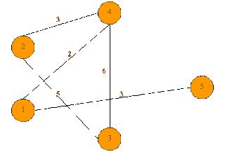
Suppose for above drawn graph (figure 5(a)) showing connected cities
Source node – 2
Destination node – 5

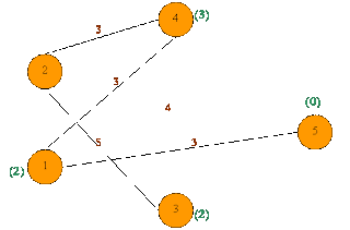
1. We need to add heuristic value to each node. Heuristic value is estimated value to reach from a given node to goal node. It should be less than or equal to actual distance.
Heuristic values added to each node for destination node 5 is shown below in figure 5(b).

Figure 5(b)

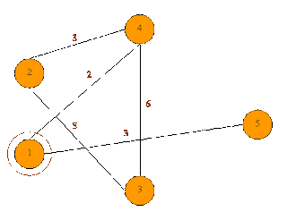
2. Source Node is Node 2. On pressing any key, it is highlighted with another round of red colour as shown in figure 5(c).

Figure 5(c)

3. The Child nodes or the connected nodes to Node 2 are Node 4 (heuristic value 3) and Node 3 (heuristic value 2). A* uses the sum of the heuristic value and actual distance from source node to explore next node.

Cost to reach Node 3 is 5 (actual distance) + 3 (heuristic value) = 8
Cost to reach Node 4 is 3 + 3 = 6

The cost to reach node 4 is less than the cost to reach node 3.So next explored node will be 4 as shown in figure 5(d).

Figure 5(d)

4. The connected nodes to Node 4 are Node2, Node 3 and Node 1. Same as Best first Search, it will also not consider visited nodes. So we left with Node 1 and Node 3.

Cost to reach node 1 is 6 (actual distance from source node) + 2 (heuristic value) = 8
Cost to reach node 3 is 7 (actual distance from source node) + 2 (heuristic value) = 9

It is clear that next node to explore is Node 1 as shown in figure 5(e).

Figure 5(e)

5. Node 1 has child nodes Node 4 and Node 5. Node 5 is having 0 heuristic value, which shows it is destination node. So it is next visited node as shown in figure 5(f).

Figure 5(f)

Hence Destination Node 5 is found. So search is complete.

NB: The system displays the path from destination node to source node. It first checks for the shortest path route and then displays nodes in reverse direction.

Best First Search

Suppose the following graph is drawn showing interconnected cities. It is a two way graph. A person can move in any direction like from vertex 2 to vertex 4 or from vertex 4 to vertex 2. An edge tells the distance between two connected cities. Different search algorithms use different strategies to find the path from source node to destination node.

Figure 4(a)

Best First Search

Best First Search is abbreviated as BEFS. It is an informed search. It uses heuristic function (i.e. estimated value to reach from a given node to goal node) to find the shortest distance from source node to destination node.

Suppose for above drawn graph (figure 4(a)) showing connected cities
Source node – 2
Destination node – 5

1. We need to add heuristic value to each node. Heuristic value is the estimated value to reach from a given node to the goal node. It should be less than or equal to actual distance. Heuristic values added to each node for destination node 5 is shown below in figure 4(b).

Figure 4(b)

2. Source Node is Node 2. On pressing any key, it is highlighted with another round of red colour as shown in figure 4(c).

Figure 4(c)

3. Child nodes or connected nodes to Node 2 are Node 4 (heuristic value 3) and Node 3 (heuristic value 2). Node 3 is having less heuristic value so it explores next as shown in figure 4(d). Although actual distance to reach Node 3 is more than distance to reach Node 4 but it does not consider actual distances at all.

Figure 4(d)

4. It does not consider visited nodes again. Like for Node 3, Child nodes are Node 2 (heuristic value 4) and Node 4 (heuristic value 3). Here heuristic value of Node 4 is less than heuristic value of Node 2, so it is explored next as shown in figure 4(e). Suppose even if heuristic value of Node 2 is less, still it will consider Node 4 because Node 2 is visited node.

Figure 4(e)

5. Node 4 has two child nodes Node 1 and Node 3. Here both Node 1 and Node 3 are having same heuristic value with value 2. But Node 3 is already visited node, so Node 1 will be visited next.

Even if there are two unvisited nodes having same heuristic value, then it works in increasing order. Node lesser in number will explore first. Suppose there are two unvisited nodes Node 2 and Node 4 having same heuristic value, Node 2 will be explored than Node 4.
So here next visited node is Node 1 as shown in figure 4(f)

Figure 4(f)

6. Node 1 has child nodes Node 4 and Node 5. Node 5 is having 0 heuristic value, which shows it is destination node. So it is next visited node as shown in figure 4(g)

Figure 4(g)

Hence Destination Node 5 is found. So search is complete.

Best First Search finds the solution in very less time. But we can see from above search that solution found is not always optimal. Path searched by Best First Search to reach from source Node 2 to destination Node 5 is 2 -> 3 -> 4 -> 1-> 5; total actual distance is 5+4+3+3 = 15

For path 2 -> 4 -> 1 -> 5; total distance is 3+3+3 = 9 which is lesser than path found by Best First Search.

NB: The system displays the path from destination node to source node. It first checks for the shortest path route and then displays nodes in reverse direction.

Dijkstras Algorithm

Suppose the graph (figure 3(a)) is drawn showing interconnected cities. It is a two way graph. A person can move in any direction like from vertex 2 to vertex 4 or from vertex 4 to vertex 2. An edge tells the distance between two connected cities. Different search algorithms use different strategies to find the path from source node to destination node.

Figure 3(a)

Dijkstra’s Algorithm

Dijkstra’s Algorithm is a special form of Breadth First Search. Dijkstra’s Algorithm finds the shortest distance from the source node to the destination node. It is also known as Single Source Shortest Path. It can find shortest distance from a single source point or source node to any destination node. Like Breadth First Search, it also searches level by level for destination node. It looks for shortest distance from one node to another. It stores distance from any current node to source node, till it does not find destination node with shortest distance.

Suppose for above drawn graph (figure 3(a)) showing connected cities

Source node is 1
Destination node is 5

1. On pressing any key, Source Node 1 gets highlighted with red colour another circle as shown in fig 3(b).

Figure 3(b)

2. Same as Breadth First Search, it looks for child nodes of parent node Node 1. Node 4 and Node 5 are child nodes of Node1. Node 5 is directly connected Node and there is no other way to reach Node 5. Hence this is the only and shortest distance to reach Node 5. So in Dijkstras Node 5 get explored next as shown in figure 3(c).

Figure 3(c)

Hence Node 5 is destination node. So Search is complete.

In Dijkstras Algorithm, it does not explore all nodes like in Breadth First Search. Only nodes which are used to reach from source node to destination node having shortest path are explored. It saves a lot of space.

NB: The system displays the path from destination node to source node. It first checks for the shortest path route and then displays nodes in reverse direction.

Breadth First Search

Suppose the graph (figure 1(a)) is drawn showing interconnected cities. It is a two way graph. A person can move in any direction like from node 2 to node 4 or from node 4 to node 2. An edge represents the distance between two connected cities. Different search algorithms use different strategies to find path from source node to destination node.

Figure 2(a)

Beadth First Search (BFS)

BFS works level by level. In Breadth First Algorithm contrast to Depth first Search, all the child nodes of a parent node are explored before moving to next level and then further child nodes of these explored nodes until a goal node is found.

Suppose for above drawn graph (figure 2(a)) showing connected cities

Source node is 1
Destination node is 5

1) Source node is Node 1. On pressing any key, it shows Node 1 with highlighting colour another round as shown in figure 2(b)

Figure 2(b)

2. Looks for child nodes of Parent Node 1. Node 4 and Node 5 are child nodes. It works in increasing order like Node 1 then Node 2 then Node 3, if Node 1, Node 2 and Node 3 are children node of any Parent node. So here Node 4 is explored first as shown in figure 2(c).

Figure 2(c)

3. In breadth First Search, all the child nodes of a node are explored at a level. So another child Node of Node 1 is Node 5. Hence Node 5 is explored after Node 4 as shown in figure 2(d).

Figure 2(d)

Hence Node 5 is destination node. So Breadth First Search is complete.

Here you can see that Breadth First Search takes lesser time than Depth First Search. Breadth First Search is very useful if destination node lies at upper levels as there is no need to go till very deep level. It saves time and storage requirement both.

Depth First Search

Suppose the graph (figure 1(a)) is drawn showing interconnected cities. It is a two way graph. A person can move in any direction like from vertex 2 to vertex 4 or vertex 4 to vertex 2. An edge tells distance between two connected cities. Different search algorithms use the different strategies to find the path from source node to destination node.

Figure 1(a)

DEPTH FIRST SEARCH

Depth First Search algorithm goes deeper and deeper at each step. For a search tree, starting from source node taken as parent node explore the first most child node ( nodes are in increasing order, node having lowest number is taken as first most child) then further first most child of child node and soon till when destination node is found or it get stuck with no child node further.

Let us say for above graph figure 1(a)
Source node - 1
Destination node – 5

1. On pressing any key it starts with source node that is Node 1. It is shown by another round of red colour on particular node as shown in figure 1(b)

Figure 1(b)

2.Node 1 has two child or neighbour nodes Node 4 and Node 5. As DFS go for the first most child, it explores Node 4 as shown in figure 1(c)

Figure 1(c)

3.Further Node 4 behaves as parent node. It looks for child node. Node 2 and Node 3 are child or neighbour nodes of Node 4. Again as Node 2 is first most child, it is explored next as shown in figure 1(d)

Figure 1(d)

4. After Node 2, Node 3 explores as the first most child as shown in figure 1(e) but node 3 has no unvisited child nodes so here search gets stuck to move more deeply. So here concept of backtracking works.

Figure 1(e)

Backtracking is a concept according to which if search reaches to dead end or leaf node, search goes back to previous explored node or can say previous execution.

In above example, Search gets stuck at Node 3. Node 3 does not have any unvisited child node so Node 3 is known as dead end. Here using backtracking concept search goes back to Parent node of Node 3 that is Node 2. But both child nodes Node 3 and Node 4 of Node 2 are already visited. It backtracks to Node 4 as this is parent node of Node 2 and further back tracks to Node 1. Node 1 has two child nodes Node 4 and Node 5. Node 4 is already visited; next Node 5 is explored as shown in figure 1(f)

Figure 1(f)

Node 5 is destination node. Hence Depth First Search completed.